Optimization

Gradient Descent (2/2)

Theory

There are three main variants of gradient descent: Batch GD (uses all data), Stochastic GD (uses one sample), and Mini-batch GD (uses small batches). Advanced optimizers like Adam and RMSprop adapt learning rates per parameter for faster convergence.

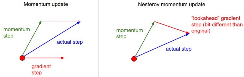
Visualization

Mathematical Formulation

Variants:
• Batch GD: Uses all training data
• Stochastic GD: Uses one sample per iteration  
• Mini-batch GD: Uses batches of data

Adam Optimizer:
mt = β₁mt-1 + (1-β₁)gt
vt = β₂vt-1 + (1-β₂)gt²
θ = θ - α·mt/√(vt + ε)

Code Example

import numpy as np

def adam_optimizer(X, y, theta, alpha=0.001, 
                   beta1=0.9, beta2=0.999, 
                   epsilon=1e-8, iterations=1000):
    """Adam Optimizer"""
    m = len(y)
    mt = np.zeros_like(theta)  # First moment
    vt = np.zeros_like(theta)  # Second moment
    
    for t in range(1, iterations + 1):
        gradient = (1/m) * X.T.dot(X.dot(theta) - y)
        
        # Update moments
        mt = beta1 * mt + (1 - beta1) * gradient
        vt = beta2 * vt + (1 - beta2) * (gradient ** 2)
        
        # Bias correction
        mt_hat = mt / (1 - beta1 ** t)
        vt_hat = vt / (1 - beta2 ** t)
        
        # Update parameters
        theta = theta - alpha * mt_hat / (np.sqrt(vt_hat) + epsilon)
    
    return theta

# Example
X = np.random.randn(100, 5)
y = X.dot(np.array([1, 2, 3, 4, 5])) + np.random.randn(100) * 0.1
theta = np.zeros(5)

theta_adam = adam_optimizer(X, y, theta)
print(f"Optimized parameters: {theta_adam}")

Gradient Descent (1/2)

Perceptron Learning Algorithm